A GENERAL TEST-BED FOR RECURSIVE SUBSTRUCTURING
IN STRUCTURAL DYNAMICS SIMULATION
BY
LLOYD VAN WARREN
B.S., University of Illinois, 1981
THESIS
Submitted in partial fulfillment of the requirements for
the degree of Master of Science in Aeronautical and Astronautical
Engineering
in the Graduate College of the
University of Illinois at Urbana-Champaign, 1983
Urbana, Illinois
© Copyright by
Lloyd Van Warren
1983
ACKNOWLEDGMENTS
I would like to first acknowledge the continual support and encouragement
of my wife, Lynn Mittelstaedt-Warren. Also to be thanked is my advisor, Dr.
Arthur L. Hale, who endured my ideas and absorption of finite element theory
with patience. Thanks also goes to Dr. Harry H. Hilton, head of the department,
for permitting me the opportunity to study aeronautical and astronautical engineering
at the graduate level, and proceed headlong into computer science in the process.
My appreciation is also extended to Wayne "J.W." Hamilton and
Patrick Kane who took me under their wings and enlightened me in the ways
of UNIX. Also the kind cooperation of Debbie Hudson, Mike Randal,
Larry Sautter, and George Badger of Computing Services Office, who enabled
me to continue to have access to a wonderful programming environment for developing
the programs described herein. Also due thanks are Turner Whitted and David
Weimer, after whose 'Raster Graphics Software Test-bed' this 'Finite Element
Test-bed' is patterned and who kindly provided me with high quality raster
graphics software. The lectures and work of L. A. Lopez that helped me to
understand the deeper software engineering problems in finite element analysis
are also appreciated.
The financial support of the National Science Foundation via
Grant No. DME-8105535 is also much appreciated.
TABLE OF CONTENTS
| LIST OF TABLES *
LIST OF FIGURES *
CHAPTER 1 INTRODUCTION *
1.1 PRELIMINARY REMARKS *
1.2 SUBSTRUCTURING *
1.3 INTROSPECTION *
1.4 OBJECTIVES *
CHAPTER 2 RECURSIVE SUBSTRUCTURING IN DYNAMIC ANALYSIS
*
2.1 INTRODUCTION *
2.2 EIGENSOLUTION BY SUBSPACE ITERATION *
2.3 A RECURSIVE ASSEMBLY PROCEDURE WITH REDUCTION *
2.4 RECURSIVE SUBSPACE ITERATION *
2.5 DISTRIBUTED VS. CENTRALIZED SOLUTION CONTROL *
CHAPTER 3 ATTRIBUTE MODELING *
3.1 INTRODUCTION *
3.2 OBJECT ATTRIBUTES *
3.3 ENVIRONMENT ATTRIBUTES *
3.4 ANALYSIS REQUESTS ATTRIBUTES *
CHAPTER 4 DATA STRUCTURES DESIGN *
4.1 INTRODUCTION *
4.2 OBJECT DESCRIPTION *
CHAPTER 5 DESIGN OF PROBLEM SPECIFICATION LANGUAGE *
5.1 INTRODUCTION *
5.2 GENERAL CONSIDERATIONS *
5.3 EVOLUTION OF GRAMMAR DESIGN *
5.4 OBJECT SPECIFICATION *
5.5 ENVIRONMENT SPECIFICATION *
5.6 ANALYSIS REQUESTS SPECIFICATION *
5.7 METHODOLOGY SPECIFICATION *
5.8 TOOLS FOR GRAMMAR IMPLEMENTATION *
CHAPTER 6 ILLUSTRATIVE EXAMPLES *
CHAPTER 7 CONCLUSIONS *
BIBLIOGRAPHY *
|
LIST OF TABLES
TABLE 2.1 SOLUTION METHODOLOGY STRATEGIES *
TABLE 4.1 RECURSIVE OBJECT DESCRIPTION FORMAT *
TABLE 4.2 TOPOLOGY DESCRIPTION FORMAT *
TABLE 4.3 NODAL DESCRIPTION FORMAT *
TABLE 4.4 NUMERICAL DESCRIPTION FORMAT *
TABLE 4.5 STATES DESCRIPTION FORMAT *
TABLE 4.6 MATERIALS DESCRIPTION FORMAT *
TABLE 5.1 CONSTRAINT COEFFICIENT MATRIX *
TABLE 5.2 METHODOLOGY ALTERNATIVES * |
LIST OF FIGURES
FIGURE 2.1 THE METHODOLOGY TREE *
FIGURE 5.1 PROBLEM REPRESENTATIONS *
FIGURE 5.2 INPUT METHODS *
FIGURE 5.3 WIDGET *
FIGURE 5.4 FRAMISE *
FIGURE 5.5 BAR OBJECT *
FIGURE 5.6 PLATE OBJECT *
FIGURE 5.7 QUAD OBJECT *
FIGURE 5.8 LEXICAL ANALYSER - PARSER INPUTS & OUTPUTS
*
FIGURE 6.1 THE 'PIECE' OBJECT *
FIGURE 6.2 THE 'PIECE2' OBJECT *
FIGURE 6.3 THE 'PIECE4' OBJECT *
FIGURE 6.4 THE 'NEWBAR10' OBJECT *
FIGURE 6.5 THE 'NEWBAR10' OBJECT FIRST NONZERO MODE *
FIGURE 6.6 THE 'NEWBAR10' OBJECT SECOND NONZERO MODE *
FIGURE 6.7 THE 'NEWBAR10' OBJECT THIRD NONZERO MODE *
FIGURE 6.8 THE 'BIGSQUARE' OBJECT *
FIGURE 6.9 THE 'BIGSQUARE' OBJECT FIRST NONZERO MODE *
FIGURE 6.10 THE 'BIGSQUARE' OBJECT SECOND NONZERO MODE
*
FIGURE 6.11 THE 'BIGSQUARE' OBJECT THIRD NONZERO MODE
* |
CHAPTER 1
INTRODUCTION
1.1 PRELIMINARY REMARKS
Simulating the dynamic response of a complex structure to its
environment requires the formulation of a suitable mathematical model of the
structure in its environment and efficient solution algorithms for calculating
the response. Also required are methods for specifying the problem in a convenient
way, and methods for viewing the results.
The finite element method provides a universal tool for formulating
mathematical models, as its pervasive use attests. The method is ideally suited
to the digital computer, the mathematical model being formulated by a computer
program. However, a complex problem's definition and its specification to
a computer system can require considerable human effort. By modeling a complex
structure as an assemblage of substructures, the human effort can be subdivided
and the total effort reduced.
1.2 SUBSTRUCTURING
To distinguish between the concepts of data structures and
engineering structures, the words 'object' and 'subobject' will be used to
mean engineering structure and substructure respectively. The word 'object'
is chosen to represent this general entity because it emphasizes the similarity
between graphical and finite element representations. The words 'data structure'
will continue to mean data structure, and the word 'substructuring' will be
used as a verb, in place of the very awkward word 'subobjecting'.
Criteria for subdividing an object usually correspond to easily
recognizable boundaries. The boundaries arise naturally during stages of design,
fabrication and manufacturing. For a given object many possible divisions
into subobjects exist. Moreover, the division can have many levels. If, at
the most fundamental modeling level, finite elements are considered as subobjects,
then a subobject at any higher level can be specified as a collection of already
defined subobjects. The result is a natural building block approach to problem
specification. The model for each subobject, starting at the lowest level,
can be formulated from its specifications and ultimately a full problem model
can be obtained.
Note that two views of substructuring are defined, namely,
1) the process of subdividing from the top down and 2) the process of successive
specification from the bottom up. Because both views are useful, it is important
that the specification process not be limited to one view or the other.
Once a problem is completely specified, the response is obtained;
hopefully, it is obtained by an efficient solution algorithm. A full finite
element model for a complex object typically possesses a large number of degrees
of freedom. The number often exceeds ten or even one hundred thousand. The
large number results from the finite element modeling process and not from
the complexity of the expected response. Therefore, a computational model
possessing a substantially reduced number of degrees of freedom is desirable,
especially if computational economy can be gained. To this end, substructuring,
possibly multileveled can be exploited. The idea is almost twenty years old
for both linear statics [PRZE63]and linear dynamics analyses [HURT65]. In
this context, substructuring is now part of a solution algorithm. The accepted
practice is to use the same division into subobjects as that chosen for problem
specification. However, a different division may be more appropriate for a
given task..
Substructuring concepts for static analyses, including computer
software implementation, are at a high level of development [NOOR78, PETE77,
DODD80].One reason is perhaps the simplicity of static analyses. Each subobject
model can be exactly reduced to its boundary degrees of freedom by static
condensation. Then, statically condensed subobjects can be assembled to form
the whole object model. For linear problems, any computational economy gained
depends on the choice of subobjects and on how many identical subobjects are
involved [NOOR78].Even if little or no economy is gained, an advantage of
substructuring in linear static analyses is simplified problem specification.
The properties of good finite element software for implementing substructuring
and easy problem specification are discussed in [SCHR79, LOPE82, DODD82].
Exact condensation of a subobject model to its boundary degrees
of freedom cannot be realized in the time domain for dynamic analyses. An
exact condensation can be performed in the frequency domain although frequency
dependent subobject coefficient matrices are introduced [BERM73]. Because
constant coefficient matrices are desirable, many approximate methods for
reducing the number of subobject degrees of freedom in the time domain have
been proposed. One alternative is to ignore the time dependence of the internal
degrees of freedom and use static condensation. Another possibility is to
represent the response of each subobject by a combination of its lower modes
of vibration. The latter technique is known as component modes synthesis [HURT65,
DOWE72, BENF71, MACN71, HINT75, CRAI77]. Component modes synthesis is a special
case of the general substructure synthesis method [HALE80, MEIR81].The general
substructure synthesis method is a Rayleigh-Ritz method, wherein the order
of each subobject is reduced before the subobjects are coupled together to
form the whole object. Finally, novel algorithms for iteratively improving
the reduced representation of each subobject in the object synthesis have
been proposed [HALE82a, HALE82b].
1.3 INTROSPECTION
This thesis builds on the general substructuring algorithms
of [HALE82a, HALE82b] for dynamic analyses by considering the "software engineering"
concepts required to implement the general substructuring algorithms. The
premise is that algorithms and their associated software implementation must
be considered together if the algorithms are to become useful tools. The reader
familiar with computer graphics will observe that the present test-bed for
recursive substructuring follows pattern set in [WHIT81].
Development of substructuring software is easiest in a proper
computational environment [LOPE82, DODD82]. The first requirement is a high
level structured programming language that has general data structuring capability
so that problem attributes can be divided into convenient conceptual groups
for easy referencing by the programmer. A second requirement is a language
that allows pointers to data to eliminate unnecessary copying and moving of
large amounts of data. A language/operating system environment that permits
dynamic allocation of memory also helps to provide for efficient use of resources
when problem solution is underway.
Because the test-bed runs in a virtual memory environment,
there is not yet much concern about how large problems are. There is interest
in only using as much memory resource as is required for the current state
of the problem. A third requirement is a software environment that possesses
a good human interface, and good software building and maintenance tools.
A data structure is the computational embodiment of any representation
scheme. For recursive substructuring it is important that all object data
structures look the same whether a simple or a complex object is being modeled.
When object data structures have the same appearance, fewer software modules
are required to solve the problem, provided the special case at the top or
the bottom level of object definition is eliminated. The price paid for this
generality in the present system is negligible. In fact, it forces the problem
to be posed in a self-consistent way that is independent of level.
Objects also have the same set of attributes whether they are
complex or simple. Little distinction is made in the test-bed between a bar
element and a complex structure with a thousand degrees of freedom. This is
accomplished economically through the use of data structures which contain
pointers to records, rather than the records themselves. For example, both
a bar element and a bridge possess the attributes of topology and material
constitution. But, a bridge is more complex topologically and materially than
a bar. In other words, it is the specific instances of the attributes that
differ in complexity. A more important difference is the fact that a bar has
no subobjects, while a bridge does. This provides a recursion termination
criterion. If an object has no subobjects, then it is an element and its mass
and stiffness matrices either already exist, or they can be found with a single
procedure call.
The fact that the same data structure is used to represent
objects regardless of the substructuring level is important because it allows
programs to be ignorant of the complexity of the entity upon which they are
currently operating. Using the same data structure at every level also has
some nice implications when writing routines that exploit the recursive nature
of the object description. There are two primary types of procedures that
occur in the test-bed, namely, those that operate on several kinds of object
data simultaneously, and those that manipulate only one kind of data. The
latter tend to be utilities such as a matrix multiplication procedure. Of
the former procedures, several important software modules in the test-bed
are recursive and they require access to many kinds of object data. A typical
recursive module takes a single argument which is a pointer to the data structure
for the object it is currently processing. The ease with which passing pointers
allows access to all of an object's data cannot be overemphasized.
Next, the test-bed user can specify problems via a problem
specification language that is similar in its syntax to the Lisp language.
Using a Lisp-like syntax has a couple of advantages. First, it eliminates
ambiguities in the grammar of the problem specification language. Second,
it allows an easy transition from the present test-bed to one that is written
in Lisp. The power of Lisp as a language for problem specification and for
computation is skillfully discussed in [REYN78, REYN82]. In his Actor/Scriptor
Animation System (ASAS) Reynold's goes at least one order of magnitude past
current computer graphics systems is his ability to define complex objects,
and to define and manipulate geometric and photometric relationships between
objects.
Finite element analysis and computer graphics share several
important characteristics. They are both areas which tend to require the user
to express complex topologies and object relationships. Both also attempt
to model complementary segments of the real world and both activities tend
to be compute bound. In computer graphics, the expense is in generation of
shaded three-dimensional images for animated scenes, while in finite element
analysis the expense is in the calculation of an object's response history.
1.4 OBJECTIVES
The goal of this work was to build a finite element test-bed
for the evaluation of substructuring and order reduction algorithms. The goal
of these techniques is reducing the cost of finding the response of an object
to its environment. An easily reconfigurable test-bed has been constructed
that allows many new and novel algorithms to be tested in a straightforward
fashion.
CHAPTER 2
RECURSIVE SUBSTRUCTURING IN DYNAMIC ANALYSIS
2.1 INTRODUCTION
A recursive procedure is defined for purposes here as a procedure
that can repeat itself until a specified condition is met. If a given object
is considered to be made of subobjects which are themselves made of subsubobjects,
etc, then object specification is recursive. Herein, the recursion terminates
when an object's data is defined only via a procedure call. The procedure
call is usually associated with a basic finite element. However, the test-bed
does not require the object to be a basic finite element and very complex
procedures can be invoked. Recursive substructuring can be further justified
by noting a number of popular algorithms in numerical analysis and computer
graphics that also lend themselves well to recursion. Polynomial root finding,
adaptive quadrature for numerical integration, Warnock's hidden line algorithm
which recursively divides and conquers, and Catmull's recursive bicubic patch
subdivision are four examples [COHE82].
Making objects' definitions similar at every level has some
very desirable consequences, both for the user defining the problem and for
the software modules processing the problem. This idea is not new to finite
element programs; the POLO FINITE static analysis program [DODD80] is an example.
First, from a software point of view, a given module does not need to know
explicitly all of an object's complexity or at what level in the object definition
it operates. A software module or 'processor' can be given the data for an
object and then call itself when appropriate for each subobject of that object.
Second, from a problem input point of view an object is defined once. The
defined object can be used as a subobject of another object and it can be
used at any level.
This 'building block' process can be very powerful. It allows
the user to rapidly specify complicated topologies with little effort. In
addition, work done one day defining objects is useful on another when the
same object is needed again.
Because this thesis emphasizes the test-bed itself rather than
the large variety of substructuring computational algorithms that it can implement,
this chapter is intended to be only illustrative of recursive substructuring.
For simplicity, the eigenvalue problem for undamped free vibration is chosen
along with the subspace iteration method for obtaining the eigensolution.
2.2 EIGENSOLUTION BY SUBSPACE
ITERATION
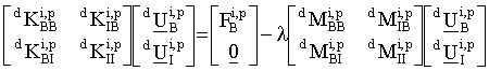
The natural frequencies and natural modes of vibration for
a complex object are obtained by solving the eigenproblem:
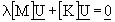 (2.1)
(2.1)
where:
 and
and  are
the N by N symmetric mass and stiffness matrices of the object,
are
the N by N symmetric mass and stiffness matrices of the object,
 is the N
dimensional displacement vector and
is the N
dimensional displacement vector and  is
an eigenvalue.
is
an eigenvalue.
For objects with a large number of degrees of freedom, the response
usually involves the first few modes only. Rather than solve the full order
eigenproblem for all modes, it is necessary to obtain only the lower modes.
The mass and stiffness matrices can be reduced, perhaps by several orders of
magnitude, via the Rayleigh-Ritz method and the reduced eigennproblem solved.
The resulting eigensolution only approximates the actual lower modes. The accuracy
of the approximation can by increased by generating improved Ritz trial vectors
and repeating the reduction process iteratively. This procedure is known as
'subspace iteration' and is described along with several of its novel variants
in [HALE82b]. Other references for the classical subspace iteration method are
[PARL80, BATH82, JENN77, MEIR80].
The classical subspace iteration method is described by the
following steps. In the following development please note that the superscript
does not imply exponentiation, but rather an iteration number.
1) Rayleigh-Ritz Step
a) Represent an eigenvector  at
iteration p as the sum:
at
iteration p as the sum:
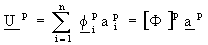 (2.2)
of n independent trial vectors
(2.2)
of n independent trial vectors 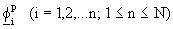 and
form the n dimensional reduced eigenvalue problem:
and
form the n dimensional reduced eigenvalue problem:
 (2.3)
(2.3)
b) Solve (2.3) for the n computed eigenvalues  and
the associated eigenvectors
and
the associated eigenvectors  (r
= 1, 2, ..., n).
(r
= 1, 2, ..., n).
c) Compute the associated approximate eigenvectors
 (2.4)
2) The Subspace Improvement Step
a) Generate n improved trial vectors
(2.4)
2) The Subspace Improvement Step
a) Generate n improved trial vectors  by
solving
by
solving
 (2.5)
Next, it is informative to consider a choice of Rayleigh-Ritz
trial vectors in conjunction with a modification to the above algorithm. The
motivation is the theme of treating objects on all levels in the same way. Therefore,
the object considered above should be treated in the same way as an object dO
at recursion depth d. Consider an object at recursion depth d,
denoted by dO, to be divided in some
convenient way into m subobjects doi,
i = 1, 2, ..., m. It is understood that each subobject can be
further subdivided, and the process continues until the recursion terminates.
(2.5)
Next, it is informative to consider a choice of Rayleigh-Ritz
trial vectors in conjunction with a modification to the above algorithm. The
motivation is the theme of treating objects on all levels in the same way. Therefore,
the object considered above should be treated in the same way as an object dO
at recursion depth d. Consider an object at recursion depth d,
denoted by dO, to be divided in some
convenient way into m subobjects doi,
i = 1, 2, ..., m. It is understood that each subobject can be
further subdivided, and the process continues until the recursion terminates.
Each subobject doi
acts as part of the parent object dO
and the eigenproblem for dO is described
within doi by the equations:
 (2.6)
(2.6)
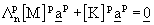
where  and
and  are the
  bysymmetric
mass and stiffness matrices,
bysymmetric
mass and stiffness matrices,  is
the dimensional displacement
vector and
is
the dimensional displacement
vector and  is an eigenvalue.
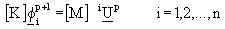
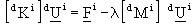
During the assembly process only those degrees of freedom associated with
the boundary of the object are transformed. The eigenproblem at iteration
p for the object doi
at recursion depth d is posed in terms of the following partitioned
matrix equations [HALE82b]:
is an eigenvalue.
During the assembly process only those degrees of freedom associated with
the boundary of the object are transformed. The eigenproblem at iteration
p for the object doi
at recursion depth d is posed in terms of the following partitioned
matrix equations [HALE82b]:
 (2.7)
(2.7)
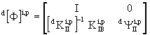 (2.8)
(2.8)
The improvement process is then given by:
 (2.9)
(2.9)
For considerably more detail see [HALE82b].
2.3 A RECURSIVE ASSEMBLY PROCEDURE
WITH REDUCTION
All finite element programs exploit the ease with which complex
mass and stiffness models can be built by assembling the submatrices together
into the matrix for the parent object. Because the assembly process is well
known and is inherently hierarchical, see [BATH82, COOK81, MEIR80, ZIEN77],
it is a good example of a recursive procedure. Explicitly, recursive assembly
can be described by the following general procedure:
procedure assemble (A: Object A)
begin
for (each subobject ai
in A) do
begin
if (ai
mass and stiffness 'formed state' is NO)
begin
assemble(ai)
end
end
if (A mass and stiffness 'formed state' is NO)
begin
get space for mass, stiffness, and right hand side
end
if (A is an element)
begin
if (A mass and stiffness 'formed state' is NO)
call A's element procedure
end
else
begin
for (each subobject ai
in A) do
begin
if (ai
is an element)
call element procedure for ai
put ai mass, stiffness,
and right hand side into A's
end
end
set A 'formed state' to YES
if (A has more than permitted internal degrees of freedom)
begin
get space for reduced mass, stiffness, and right hand
side
form the desired number of Rayleigh-Ritz basis vectors for
reduction
reduce A's mass, stiffness right hand side
set A reduction state to YES
end
end
This assembly procedure starts with the parent object and continues
until all the children on all levels are processed. It is important to note
the appearance of the Rayleigh-Ritz reduction process in the bottom if
clause of procedure assemble. When reduction is incorporated into the
assembly process, the number of degrees of freedom of objects on any level can
be regulated uniformly and automatically. The same assembly procedure is used
whether reduction of an object is desired or not. If reduction is not desired,
the number of permitted internal degrees of freedom need only be specified as
a number larger than the number of degrees of freedom in the object.
2.4 RECURSIVE SUBSPACE ITERATION
When the concept of subspace iteration is combined with recursive
assembly and reduction on several levels of a problem, a host of possible
multi-level iterative algorithms arise [HALE82b]. Note that in the following
discussion, function returns a value while a procedure does
not.
One procedure for 'multi-Ritz' is given below:
assemble(A)
procedure multi_Ritz (A: Object A)
begin
while (converged is NO)
begin
solve eigenproblem for A
converged = recur_iterate(A)
end
end
The function for 'recur_iterate' is then:
function recur_iterate (A: Object A)
begin
if(object A's mass and stiffness 'reduction' state
is YES)
begin
if(object A's eigenproblem not converged)
begin
expand A's reduction basis vectors
improve A's reduction basis vectors
reduce A's mass, stiffness and right hand side using basis
vectors
return(NO)
end
end
if(reduction occurs below A)
begin
if(A is reduced)
begin
expand A's reduction basis vectors
end
for (each subobject ai
in object A) do
begin
if (ai
is reduced or has reduced subobjects)
begin
pass A's eigenvectors downward to ai
a_yes_no = recur_iterate(ai)
if(a_yes_no is NO)
begin
A_yes_no = NO
end
end
if(A_yes_no is NO)
begin
reassemble(A)
return(NO)
end
end
return(YES)
end
The procedure reassemble is similar to assemble and
is omitted for brevity.
2.5 DISTRIBUTED VS. CENTRALIZED
SOLUTION CONTROL
There are many alternatives to monitoring and controlling the
flow of the solution in a dynamics problem analysis. The phrase 'solution
control' means the choice of methodologies or procedures to invoke when the
problem is in a state where there is more than one way to proceed to a solution.
Optimally, the path through the methodology options tree that minimizes the
cost of solution is desired. Finding the optimal solution path is beyond the
scope of this work. It is nevertheless an interesting problem and it represents
the 'right' approach to 'solution control'.
Given a set of basic procedures that can be used to perform
an engineering analysis, there are several alternatives. The basic procedures
might include assembly, reduction, constraint imposition, etc.. The procedures
can be viewed as operators in the mathematical sense.
Presently, a distributed solution controller implemented via
a set of solution state flags is used. Each procedures looks at the object
state flags while the problem is being solved and makes appropriate decisions.
The optimum methodology should be chosen on the basis of minimum cost. If
estimating the cost of subproblem solution is expensive with respect to solving
the subproblem this fact should be returned to the calling procedure which
could then make a decision about whether to go ahead and solve the subproblem.
This amounts to estimating the cost of estimating the cost. Some options that
can be chosen for three typical finite element operators are listed in Table
2.1.
TABLE 2.1 SOLUTION METHODOLOGY
STRATEGIES
|
recursive operator
|
possible main strategy
|
possible sub-strategy
|
assemble
|
all at once
on the fly
|
breadth first
depth first
breadth first
depth first
|
reduce
|
all at once
on the fly
|
breadth first
depth first
breadth first
depth first
|
constrain
|
all at once
on the fly
|
breadth first
depth first
breadth first
depth first
|
There are a large number of solution paths. The options
that occur at a given step in the solution comprise a set of possible branches
which define a methodology tree (see figure 2.1).
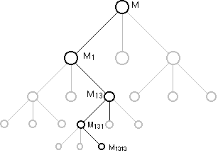
FIGURE 2.1 THE METHODOLOGY
TREE
Good controllers should attempt to reach the bottom of the
tree via the minimum cost path. It can be difficult and expensive to find
this minimum cost path; it may often be more expensive than solving the problem!
Therefore, heuristics can be used that make a good decision based on available
information. In the present setting, heuristics can be used to toggle state
flags that will determine the solution path. This idea of using heuristics
has been implemented only to a primitive degree in the current test-bed.
CHAPTER 3
ATTRIBUTE MODELING
3.1 INTRODUCTION
Engineering problems have attributes that can be drawn from
four basic categories, namely, object attributes, environment attributes,
analysis requests attributes (what answers does the user want), and methodology
attributes (how the user wants those answers to be obtained). The goal of
an analysis and its associated bookkeeping must be separated from the mathematical
model of the problem.
3.2 OBJECT ATTRIBUTES
A generalized object is a computational entity comprised of
zero or more subobjects. To construct an attribute model one must answer a
series of questions. For example, "What are the subsets that describe the
set of current interest?". Also, "What are the attributes associated with
each subset?". Finally, "What are the states associated with each of the attributes?".
Because attribute modeling is a procedure, it could be automated. Since it
can be automated, it is possible that a machine could do the attribute modeling.
If the relationships between the attributes can be extracted by a similar
set o questions, then that too could be automated. Simulating the conversation
between a person and a machine enables the attributes to be extracted in an
orderly and self-consistent fashion.
The conversation might proceed as follows:
| Machine: |
"What are the attributes of an object?" |
| Person: |
"An object has:
identification
information,
topology,
materials,
nodes,
subobjects,
an object mathematical
model." |
| Machine: |
"What are the attributes of identification information?" |
| Person: |
"Identification information has:
a name,
a number." |
| Machine: |
"What are the attributes of topology?" |
| Person: |
"Topology has:
internal topology,
external topology." |
| Machine: |
"What are the attributes of internal topology?" |
| Person: |
"Internal topology has:
a list of relationships
between subobjects." |
| Machine: |
"What are the attributes of external topology?" |
| Person: |
"External topology has:
a list of relationships between the current object and
other objects." |
| Machine: |
"What are the attributes of materials?" |
| Person: |
"Materials have:
identification
information, (machine has seen this above!)
a material
mathematical model." |
| Machine: |
"What are the attributes of nodes?" |
| Person: |
"A node has:
identification
information, (machine has seen this above!)
physical coordinates,
degrees of
freedom." |
| Machine: |
"What are the attributes of subobjects?" |
| Person: |
"A subobject has:
all the attributes
of an object" (recursive definition) |
| Machine: |
"What are the attributes of an object's mathematical
model?" |
| Person: |
"An object mathematical model
has:
mass matrices,
damping matrices,
stiffness matrices,
relational
or boolean matrices,
element procedures,
force vectors,
displacement
vectors,
velocity vectors,
acceleration
vectors,
stress vectors." |
The conversation is continued until the questions all result
in a primitive data type, such as a number or a character string. Associated
with each attribute are states of interest that could be derived from a similar
conversation. States include whether an attribute is unique or shared among
several objects and whether an attribute is defined.
3.3 ENVIRONMENT ATTRIBUTES
In addition to the description of the object itself, in finite
element analyses objects are placed in and interact with environments. Often
there is ambiguity whether certain quantities such as forces are attributes
of the object or of the environment. Because forces are associated with specific
regions of the object, they could be associated with the object. But outside
forces are really just external signals coming from the environment. Therefore,
it seems that they should be an environmental attribute rather than an object
attribute. This paradox surfaces often when one considers the 'who forces
who' question. The domain of the object upon which the force acts is definitely
an attribute of the object. The force itself, however, belongs to the external
environment.
An environment can have:
a field, e.g. temperature or body force field,
a set of forces which impose themselves on the object at
specific locations.
3.4 ANALYSIS REQUESTS ATTRIBUTES
Finally, it is necessary to configure the analysis procedures
so that requested answers are provided, hopefully with the minimum utilization
of resources.
Analysis requests have:
unknown quantities (e.g. stresses, displacements or vibrational
modes)
computational costs.
Because of the programming difficulty, this has computational
cost analysis has not been implemented.
CHAPTER 4
DATA STRUCTURES DESIGN
4.1 INTRODUCTION
Objects in environments are the what and where of engineering
problems. By listing the attributes of objects and environments, one represents
these problem entities in an orderly fashion. The attributes must also be
represented by the machine in an orderly fashion, where the machine representation
consists of a data structure.
In designing finite element software, especially easily reconfigurable
codes, it is desirable to structure the problem's data in a logical and self-consistent
way. By using a structured programming language that supports data structuring,
it is only necessary to define the data structures that group the problem
attributes in a way suitable for efficient storage, solution and coding.
Efficient storage is gained by aligning frequently referenced
quantities. This is somewhat machine dependent. As far as the data structuring
goes, efficient manipulation is obtained by minimizing the number of pointer
calculations that are necessary to reference a value. Deeply nested data structures
are to be avoided for frequently referenced items. Efficient coding is allowed
when related data items are clustered in a natural way.
When designing data structures, the difficult question of whether
to use the hierarchical, relational, or network approach to organizing the
data arises. The details of each approach to data management I well covered
in [DATE76]. In chapter 3 of [DATE 76] on data structures and operators it
is stated that "... hierarchies are obviously a natural way to model truly
hierarchical structures from the real world". This is the approach taken herein.
Nevertheless, the test-bed data structures can be cyclically linked to resemble
the network approach if need should arise. The problem with the hierarchical
approach is that it is possible to ask questions about an object that require
a search of all the branches in the hierarchy. For instance, if one wants
to know which nodes of the root object correspond to the nodes of a bottom
level object, one has to search and correlate. However, for complex objects
the cost of traversing the tree is small when compared to the cost of a complicated
problem's solution.
4.2 OBJECT DESCRIPTION
Because an object description must be compact, pointers to
records are always used at the object description level in lieu of the records
themselves. This has some nice implications when movement of data becomes
necessary. Pointers can be copied or reassigned rather than large records.
In the complete description of an object, a rather complex pointer network
is created.
In table 4.1 the attributes of an object and pointers to instances
of each attribute are recorded. Note that only pointers occur in the object
description. This allows for compactness and for ease of generalizing the
data structures while minimizing the propagation of changes to test-bed procedures.
|
TABLE 4.1
RECURSIVE OBJECT DESCRIPTION FORMAT
|
|
ATTRIBUTE
|
INSTANCED BY
|
| identification |
pointer to i.d. description
|
| topology |
pointer to topology description
|
| materials |
pointer to materials description
|
| numerical information |
pointer to numerical description
|
| states |
pointer to states description
|
| environment |
pointer to environment description
|
Table 4.2 contains the topological or connectivity information
for the object. Internal topology is recorded via the subobject list. External
topology, i.e. what objects neighbor this object, is recorded via the incidence
table.
|
TABLE 4.2
TOPOLOGY DESCRIPTION FORMAT
|
|
ATTRIBUTE
|
INSTANCED BY
|
| nodes |
a) number of nodes
b) pointer to list of pointers to node descriptions
c) list of boundary nodes |
| subobjects |
a) pointer to list of pointers
to subobject's object descriptions b) number of
subobjects |
| incidences |
pointer to incidence table |
| nodal reordering |
permutation vectors |
Table 4.3 represents the recorded attributes of a node.
|
TABLE 4.3
NODAL DESCRIPTION FORMAT
|
|
ATTRIBUTE
|
INSTANCED BY
|
| geometric coordinates |
x1, x2, x3 |
| normal direction |
nx1, nx2, nx3 |
| constraint state |
pointer to constraints |
| degrees of freedom |
pointer to vector containing
displacements, stresses, etc. |
The mathematical model for the object is contained in the numerical
data structure (table 4.4) which contains pointers to arrays of all pertinent
numerical information. Using several levels of pointers need not be slow for
numerical computations, because once a record is located, a single level pointer
to that record can be used to access and assign its contents. Test-bed routines
that deal with matrices utilize this and tend to be quite reasonable in their
execution speed.
|
TABLE 4.4
NUMERICAL DESCRIPTION FORMAT
|
|
ATTRIBUTE
|
INSTANCED BY
|
| full mass matrix |
pointer to |
| full stiffness matrix |
pointer to |
| full right hand side vector |
pointer to  |
| reduced mass matrix |
pointer to |
| reduced stiffness matrix |
pointer to  |
| reduced right hand side vector |
pointer to  |
| eigenvalues vector |
pointer to  |
| full eigenvectors matrix |
pointer to  |
| reduced eigenvectors matrix |
pointer to  |
| basis vectors |
pointer to  |
| constraint matrices |
pointer to  |
| element function pointer |
pointer to element subroutine |
| numerical states |
list of state flags |
The states description (table 4.5) is used to characterize
the object's state at a given time during the computational procedure. This
permits the use of adaptive algorithms.
|
TABLE 4.5
STATES DESCRIPTION FORMAT
|
|
FLAG
|
PURPOSE
|
| def_by_fun |
indicates if object is an element |
| formed |
indicates if object has data |
| linear |
indicates if object is linear |
| symmetric |
indicates if object has symmetric
formulation |
| reduced |
indicates if object has been
reduced |
| reordered |
indicates if object have been
reordered |
| num_replicate |
indicates if object is a numerical
replicate of another |
| num_times |
indicates number of occurrences
of object at this level |
The materials description (table 4.6) holds the object's material
properties, and provides a slot for simple or complex material models.
|
TABLE 4.6
MATERIALS DESCRIPTION FORMAT
|
|
ATTRIBUTE
|
INSTANCED BY
|
| elastic modulus |

|
| mass density |

|
The present approach has aptly been called 'pointers gone wild',
particularly because of the tracking through 3 or 4 nested levels of pointers
to pointers to pointers. The programming problem becomes on of managing the
pointer network. This can be done by associating states with each pointer
in the net. If a pointer actually points to something, i.e. space has been
allocated, then a bit can be set to indicate that it is permissible to access
the record. This idea leaves the job of checking and allocating space to active
procedures. The overhead of toggling the bit is quite small. Moreover, the
idea extends easily to the management of sparse and full matrices that are
stored in one dimensional form. Two or three bits are sufficient to know the
allocation state and the storage type for an array.
CHAPTER 5
DESIGN OF PROBLEM SPECIFICATION LANGUAGE
5.1 INTRODUCTION
There are two kinds of problem representation that are of concern:
the first is the external human representation, and the second is the internal
machine representation. A parser is required for proper translation of an
external language representation to an internal one.
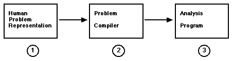
FIGURE 5.1 PROBLEM REPRESENTATIONS
These human and machine problem representations can be expanded
further:
A) Human Problem Representation
1) Pictorial Representation
2) Alphanumeric Representation
B) Machine Problem Representation
1) High Level Programming Language Rep
2) Lower Level Programming Language Rep
n) Binary Machine Language Rep
A good interface should allow interactive specification of
the engineering problem at hand via a graphic medium. The output of such an
interface would be a problem definition that could then be used by the parsing
program to generate the data required for solution of the problem.
This chapter discusses the design and implementation of a problem
specification language (PSL) that is modular, easy to use, compact and self-consistent.
Until an interactive front-end for graphic problem specifications is written,
an alphanumeric language will suffice. The language can later serve as a guide
for an interactive and graphic problem specification program (see Figure 5.1).
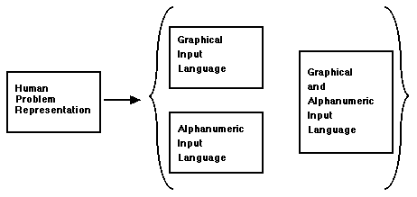 FIGURE 5.2 INPUT METHODS
The test-bed contains a problem parser that translates a language
specification into a binary form that is processed by the analysis program.
This is adequate for testing algorithms, but could be improved so that a recompile
would not be necessary to try out a new solution algorithm.
The goal is to provide an easily altered form of specifying
problems. Previous efforts in this area are described in [DODD80]. The present
goals are modularity and reasonable speed. The pitfalls of monolithic software
systems, that are avoided here are discussed in detail by Schrem [SCHR79]
and Felippa [FELI81].
5.2 GENERAL CONSIDERATIONS
Each problem requires a set of description statements that
are collected and parsed together. Object A is made of subobjects a, b, and
c, which are in turn made of subobjects, etc. Therefore, the specification
of complicated objects is hierarchical. Each object has a set of nodal coordinates
which represent a local coordinate basis. The local coordinates can be transformed
into global coordinates automatically when the object is used as a subobject
of another object. This way trouble doesn't arise when an object has subobjects
which are all replicates of each other. Complete global coordinate information
for each node, when it is needed, can be generated from coordinate transformations.
The global coordinate system is just the local coordinate system for the object
that is currently under analysis. This suggests that it may be appropriate
to solve the subobject problems in their own coordinate systems and then transform
the results only for those control points (usually nodes) which are common
both to the subobject and object itself.
There are two main approaches to problem specification that
must be permitted. In the first approach, a problem is defined by building
up from available library objects. Library objects can be elemental objects
or objects of arbitrary complexity defined in previous sessions. This is a
powerful 'bottom up' approach. In the second approach, a complex problem is
presented and it is desired to develop an accurate finite element model. This
approach is top down in that one starts with a complete problem definition.
Also to be given attention in the design of a PSL is the fact
that while an object can be very complicated internally, it often is connected
to the outside world at relatively few points. A PSL should exploit this fact
and allow the connectivity information to be expressed in terms of this fewer
number of control points.
5.3 EVOLUTION OF GRAMMAR DESIGN
Several evolutionary stages took place in designing the grammar
for the test-bed. In the first stage, specific instances of objects and environments
were listed in tables, where each table represented some attribute. In the
second, delimiters were introduced so that the problem specification could
be context free. In the third stage, the delimiters were restricted to open
and closing parentheses, and a nested list form was imposed. The final result
is a Lisp-like input grammar [WINS81].
It is interesting to explicitly discuss the evolution of the
grammar. First, the nodal coordinates a of a quad element were presented in
a table as follows:
NODES 4
|
Node
|
x
|
y
|
z
|
|
1
|
0.0 |
0.0 |
0.0 |
|
2
|
1.0 |
0.0 |
0.0 |
|
3
|
1.0 |
1.0 |
0.0 |
|
4
|
0.0 |
0.0 |
0.0 |
This simple table illustrates the presense of some important
descriptive issues. The keyword 'NODES' is an attribute label. The next line
'node x y z' is a header that establishes the format of what follows. The
header is followed by the entries themselves. In this first stage, the white
space surrounding the data was significant, i.e. formated input was used.
In the second incarnation of the grammar, a context free specification
was sought that did not depend on the concept of a line, or on the precise
nature of white space that surrounds the characters. In order to obtain an
unambiguous grammar, delimiters were introduced. The tables took the form
of chunks of programming language code. The above table was transformed to
the following:
{ NODES 4
node x y z
;
1 0.0 0.0 0.0
;
2 1.0 0.0 0.0
;
3 1.0 1.0 0.0
;
4 0.0 0.0 0.0
;
} |
The general format is expressed as follows:
{ ATTRIBUTE_KEYWORD number
header ;
data record
1 ;
data record
2 ;
' ' ' ;
data record
n ;
} |
The presense of the header is interesting because it allows
the program that parses the chunk to be 'data driven' (see [WINS81]). The
program is expected to look at the header, and then decide what should be
done with that data. This allows building some intelligence into the program
in a clean and modular way. A popular example is a program that calculates
the area of a geometric figure. The header would state whether the figure
is a square or a circle or a polygon.
After reflecting on the second version of the grammar, it became
clear that the attribute keyword could be viewed as an operator. Because a
more general grammar than the above 'C' syntax was needed, the grammar was
converted to a Lisp-like syntax. The advantage of Lisp is that, in Lisp, programs
and data have the same appearance. Lisp can also provide a consistent framework
for problem specification and solution regardless of how complicated the problem
becomes. This is because Lisp is self-consistent and possesses a sound mathematical
basis [CHUR41]. In attempting to specify problems at this level, natural language
input or a more syntactically rigorous variant of natural language was the
goal. Terry Winograd's pioneering work in natural language understanding [WINO74]
discusses a Lisp based attack of this problem. Recent examples of the expressive
power of Lisp based systems are the Animated Script and Actors system by Craig
Reynolds [REYN78, REYN82]. Finite element analysis possesses enough complexity
that the capabilities of Lisp become indispensable if progress is to continue
in reasonable time. The Lisp-like version of the table is:
( NODES 4
( node x y z )
(
( 1 0.0 0.0 0.0 )
( 2 1.0 0.0 0.0 )
( 3 1.0 1.0 0.0 )
( 4 0.0 0.0 0.0 )
)
)
where the general format of the table is:
( ATTRIBUTE_KEYWORD number
( header )
(
( data record 1 )
( data record 2 )
( ' ' ' )
( data record n )
)
)
The tables are now Lisp expressions with two arguments which
are also lists. The first list is a header and the second is the data. The
current test-bed uses this syntax. Future versions could seek to view the
attribute keyword as an operator that associates a name with a specific instance
of data of that type. The act of associating a list with a name is done in
Lisp with the setq operator. Moreover, the attribute keyword and header
serve to provide type information. The above list is of type keyword (e.g.
of type NODE in this example). A keyword type list has list structure given
by the header (e.g. 'node x y z'). It may well be that the two concepts should
be separated. The function of the headers could be stored elsewhere in a list
of templates that define the list structure. The separation could save space
when specifying a problem, although it is nice to attach the header to the
list so that the structure is known without a search. The resulting syntax
would look like:
( NODES framise_nodes
( node x y z )
(
( 1 0.0 0.0 0.0 )
( 2 1.0 0.0 0.0 )
( 3 1.0 1.0 0.0 )
( 4 0.0 0.0 0.0 )
)
)
Note that use of names as references makes it easy to refer
to an instance of an object without needless repetition. A name can also be
a number when alphameric naming would be to clumsy.
5.4 OBJECT SPECIFICATION
Problem specification consists of a list of tables. The hypothetical
object, illustrated in figure 5.3, called a widget serves as an example. In
a problem using the widget, the following object specification could be used:
 FIGURE 5.3 WIDGET
( OBJECT widget
FIGURE 5.3 WIDGET
( OBJECT widget
( TOPOLOGY
( SUBOBJECTS 3
( subobj name )
(
( 1 framise )
( 2 framise )
( 3 framise )
)
)
( NODES 3
( node x y z )
(
( 1 0.00 0.00 0.00 )
( 2 0.50 1.00 0.00 )
( 3 1.00 0.00 0.00 )
)
)
( INCIDENCES 3)
( subobj incidences )
(
( 1 1 2 )
( 2 2 3 )
( 3 3 1 )
)
)
)
)
Notice that the widget is made of a triangular ring of three
framises. Each framise appears to have two nodes, where the apparent nodes
have the coordinates listed. The description of the framise (figure 5.4) is
given below:
( OBJECT framise
( MATERIALS
( E rho )
( 1.0 1.0 )
)
( TOPOLOGY
( SUBOBJECTS 5
( subobj name )
(
( 1 beam )
( 2 beam )
( 3 plate )
( 4 beam )
( 5 beam )
)
)
( NODES 5
( node x y z )
(
( 1 0.00 0.00 0.00 )
( 2 1.00 0.00 0.00 )
( 3 0.25 0.25 0.00 )
( 4 0.75 0.25 0.00 )
( 5 0.25 -0.25 0.00 )
( 6 0.75 -0.25 0.00 )
)
)
( INCIDENCES 5
( subobj incidences )
(
(1 1 3 )
(2 1 5 )
(3 3 4 5 6 )
(4 4 2 )
(5 6 2 )
)
)
( BND_NODES 2
(1 2)
)
)
)
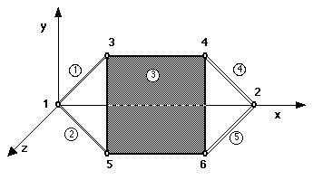 FIGURE 5.4 FRAMISE
Note that a framise actually has 6 nodes, but the first two
nodes correspond to the references made in the widget topology description
and they are specified as boundary nodes. Also the nodal coordinates are listed
with respect to a local coordinate system. Finally note the reference to an
object (the bar in this case) that has no subobjects. Indeed, the bar is considered
a finite element (see figure 5.5).
The bar topology specification is:
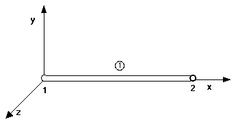 FIGURE 5.5 BAR OBJECT
( OBJECT bar
( TOPOLOGY
( NODES 2
( node x y z )
(
( 1 0.00 0.00 0.00 )
( 2 0.00 1.00 0.00 )
)
)
)
)
A plate is also listed as a subobject of the framise. The plate
(see Figure 5.6) is comprised of four quad objects and it is specified as
follows:
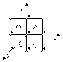 FIGURE 5.6 PLATE OBJECT
( OBJECT plate
( TOPOLOGY
( SUBOBJECTS 4
( subobj name )
(
( 1 quad ) ( 2 quad )
( 3 quad ) ( 4 quad )
)
)
( NODES 9
( node x y z )
(
( 1 -1.00 1.00 0.00 )
( 2 1.00 1.00 0.00 )
( 3 -1.00 -1.00 0.00 )
( 4 1.00 -1.00 0.00 )
( 5 0.00 1.00 0.00 )
( 6 -1.00 0.00 0.00 )
( 7 1.00 0.00 0.00 )
( 8 0.00 -1.00 0.00 )
( 9 0.00 0.00 0.00 )
)
)
( INCIDENCES 4
( subobj incidences )
(
( 1 1 5 6 9 )
( 2 5 2 9 7 )
( 3 6 9 3 8 )
( 4 9 7 8 4 )
)
)
)
)
The quad object topology specification completes the specification
of the example object. The quad (see Fig 5.7) has no subobjects and is therefore
a finite element. The quad's topology follows:
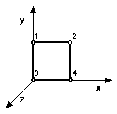 FIGURE 5.7 QUAD OBJECT
( OBJECT quad
( TOPOLOGY
( NODES 4
( node x y z )
(
( 1 0.00 1.00 0.00 )
( 2 1.00 1.00 0.00 )
( 3 0.00 0.00 0.00 )
( 4 1.00 0.00 0.00 )
)
)
)
)
An advantage of the above method of topology specification
is that subobjects can be resized or rescaled simply by changing the coordinate
description associated with the top level object. The subobject topologies
are unaffected because the topology remains the same. The 'independence',
or less formally, 'no hooks', principle is an important one. It allows changes
in one part of a problem to propagate throughout the description without requiring
all objects to be updated. Material properties can work the same way. A truss
made of steel and aluminum can be quickly modified to be composed of titanium
and aluminum by changing one entry, namely, the material definition list for
the object.
When objects possess a heterogeneous composition the subobject
material composition records can be recursively checked until a homogeneous
composition is found. For simplicity material properties are presently entered
in numerical form. However, the test-bed could easily be extended to allow
materials to be named. Then, the material properties list could be referenced
by name where needed. It remains to describe constraint specification. Herein
constraints are considered to be linear and homogeneous. The have the form
of a constraint matrix  postmultiplied
by a vector of dependent degrees of freedom.
postmultiplied
by a vector of dependent degrees of freedom.
The matrix has
constraints number of rows and degrees of freedom number of
columns. The format of constraint specification is most easily seen by example.
Assume six constraints that affect the first three nodes only. The entries
associated with the first three nodes in are
tabulated in Table 5.1:
|
TABLE
5.1 CONSTRAINT COEFFICIENT MATRIX
|
|
node 1
|
node 2
|
node 3
|
|
u1 v1 w1
|
u2 v2 w2
|
u3 v3 w3
|
|

|

|
|

|

|
|
|
|
Table 5.1 can be transformed to a more convenient form for
user input and readability by taking 3 columns at a time for each node. Then,
only data for those nodes which are actually constrained is entered. This
allows expansion to systems with many degrees of freedom per node without
packing too much information on a line. In this spirit, the information contained
in table 5.1 can be specified as follows:
( CONSTRAINTS
( NODE 1
( eqn u v w)
(
(1 1 0 0)
(2 0 1 0)
(3 0 0 1)
)
)
( NODE 3
( eqn u v w )
(
(4 1 0 0)
(5 0 1 0)
(6 0 0 1)
)
)
)
Because external constraints are usually defined at the top
level only, the multi-level description used in the topology and material
specification is unnecessary. Moreover, sparse matrix storage scheme can be
used to represent the constraint matrix if it grows too large.
5.5 ENVIRONMENT SPECIFICATION
Environment specification is not yet as well developed as object
specification. Attributes of the environment are things such as point and
distributed loads, thermal loads, and body forces such as gravity and electromagnetic
forces. The environment could also be time and space dependent. The widget
subjected to static external point loads serves as a simple environment specification
example:
( ENVIRONMENT widget
( POINT_LOADS
( node fx fy fz )
(
(1 1.0 1.0 3.0 )
(2 1.0 2.0 3.0 )
(3 1.0 1.0 3.0 )
)
)
)
5.6 ANALYSIS REQUESTS SPECIFICATION
A problem specification could also contain analysis requests,
i.e. the kind of analysis the user wants to be performed. Quick changes in
the problem are thereby permitted just by changing the specification. Analysis
requests for a widget problem might look like:
( WIDGET_ANALYSIS_REQUESTS
( QUANTITIES
displacements
velocities
accelerations
stresses
eigenvalues
)
)
( ACTIVE_PROBLEM_DESCRIPTIONS
( ATTRIBUTE
DESCRIPTION ACTIVE OVER TIME )
(
( object widget obj ALL )
( environment widget_1_env 0.0 to 10.0 sec. )
( environment widget_2_env 10.0 to 12.0 sec. )
( methodology widget_how 10.0 to 12.0 sec. )
)
)
5.7 METHODOLOGY SPECIFICATION
Finally, several functions fall exclusively into the category
of methodolgy requests. This area is the least developed. Presently, different
solution methods are obtained by rewiring the test-bed, i.e. rearranging or
coding new routines and recompiling. User specification of the solution methods
via the grammar would be nice. Once a good procedure for a family of problems
was obtained, it could be saved in a library like any other specification.
Possible alternatives are shown in Table 5.2.
|
TABLE 5.2 METHODOLOGY
ALTERNATIVES
|
|
Operator
|
Method
|
Solution Or Time Step
|
|
reduce
|
depth first
|
solution stepping relation
|
|
constrain
|
breadth first
|
time stepping relation
|
|
assemble
|
binary region splitting
|
local error tolerance relation
|
|
reassemble
|
other region splitting
|
local error toleratnce realtion
|
5.8 TOOLS FOR GRAMMAR IMPLEMENTATION
Once the grammar was designed two powerful software tools were
used to generate the code that performs the input language lexical analysis
[LESK75] and parsing [JOHN78]. The relationships for the grammar were specified,
and this grammar specification was used to generate the parsing program via
a compiler-compiler.
The primary job of the parser is to take action based on recognized
relationships. A separate program is used to actually recognize the incoming
expressions. The program that does this recognition or 'lexical analysis'
identifies defined entities known as 'tokens'. An example of a token might
be a delimiter such as a left or right parenthesis, or a keyword such as OBJECT,
or perhaps TOPOLOGY. Other examples of tokens (also known as terminal symbols)
that would be passed to the parser might include a numerical value such as
a nodal coordinate, or an object name. When tokens are then passed to the
parser, action is taken by the parser to allocate and initialize data structures
that contain problem information. The usage of these software tools is discussed
in "Yacc: Yet Another Compiler-Compiler" [JOHN78] and "Lex - A Lexical Analyzer
Generator" [LESK75].
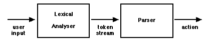 FIGURE 5.8 LEXICAL ANALYSER
- PARSER INPUTS & OUTPUTS
FIGURE 5.8 LEXICAL ANALYSER
- PARSER INPUTS & OUTPUTS
CHAPTER 6
ILLUSTRATIVE EXAMPLES
The work described herein resulted in a functioning test-bed
in which new finite element and substructuring algorithms may be evaluated.
Several examples have been run using the test-bed. The recursive substructuring
algorithm listed in Chapter 2 was used. The trial element was a bar with 2
degrees of freedom per node. The 'stick plots' of several objects, their object
descriptions and their associated frequencies of free vibration are listed
below. First we start with a 'piece' object that is made of several bars:
( PROBLEM
( OBJECT piece
( TOPOLOGY
( SUBOBJECTS 4
( subobject name)
(
( 0 bar ) ( 1 bar ) ( 2 bar ) ( 3 bar )
)
)
( NODES 4
(
(0 0.00 0.00 0.00)
(1 0.00 0.50 0.00)
(2 1.00 0.00 0.00)
(3 1.00 0.50 0.00)
)
)
( INCIDENCES 4
( subobj incidences)
(
(0 0 1) (1 0 2) (2 1 3) (3
1 2)
)
)
)
)
)
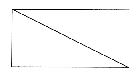 FIGURE 6.1 THE 'PIECE' OBJECT
Then we hook these together to form an new object called a
'piece2':
( PROBLEM
( OBJECT piece2
( TOPOLOGY
(NODES 6
(node x y z)
(
(0 0.00 0.00 0.00)
(1 0.00 0.50 0.00)
(2 1.00 0.00 0.00)
(3 1.00 0.50 0.00)
(4 2.00 0.00 0.00)
(5 2.00 0.50 0.00)
)
)
( SUBOBJECTS 2
( subobj name)
( ( 0 piece) ( 1 piece)
)
)
( INCIDENCES 2
( subobj incidences )
(
( 0 0 1 2 3 )
( 1 2 3 4 5 )
)
)
( BND_NODES 4 (0 1 4 5) ) )
)
)
)
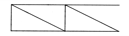 FIGURE 6.2 THE 'PIECE2' OBJECT
Then we add these to form an new object called a 'piece4':
( PROBLEM
( OBJECT piece4
(TOPOLOGY
( SUBOBJECTS 2
( subobj name )
( ( 0 piece2) ( 1 piece2)
)
)
( NODES 6
( node x y z)
(
( 0 0.00 0.00 0.00)
( 1 0.00 0.50 0.00)
( 2 2.00 0.00 0.00)
( 3 2.00 0.50 0.00)
( 4 4.00 0.00 0.00)
( 5 4.00 0.50 0.00)
)
)
( INCIDENCES 2
( subobj incidences )
(
(0 0 1 2 3)
(1 2 3 4 5)
)
)
( BND_NODES 4 (0 1 4 5) )
)
)
)
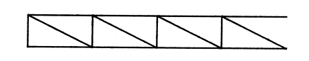 FIGURE 6.3 THE 'PIECE4' OBJECT
These are combined to form a 'newbar10':
( PROBLEM
( OBJECT newbar10
( TOPOLOGY
( SUBOBJECTS 7
( subobj name )
(
( 0 bar) ( 1 bar) (
2 piece4) ( 3 piece4) (
4 bar) ( 5 bar) ( 6 bar)
)
)
( NODES 8
( node x y z )
(
( 0 -1.00 0.25 0.00)
( 1 0.00 0.00 0.00)
( 2 0.00 0.50 0.00)
( 3 4.00 0.00 0.00)
( 4 4.00 0.50 0.00)
( 5 8.00 0.00 0.00)
( 6 8.00 0.50 0.00)
( 7 9.00 0.25 0.00)
)
)
( INCIDENCES 7
( subobj incidences )
(
(0 0 1)
(1 0 2)
(2 1 2 3 4)
(3 3 4 5 6)
(4 5 6)
(5 5 7)
(6 6 7)
)
)
( BND_NODES 2 (0 7) ) )
)
)
)
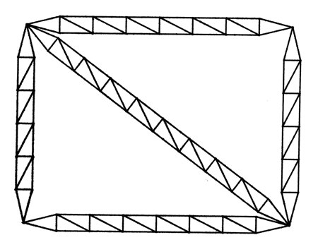
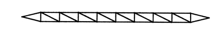 5 levels of recursion
FIGURE 6.4 THE 'NEWBAR10' OBJECT
5 levels of recursion
FIGURE 6.4 THE 'NEWBAR10' OBJECT
Now before building further we can do an eigenvalue problem
and observe the modes of free vibration:
 w2 = 1.937 x 10⁻³
s-2
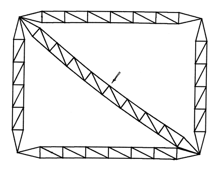
FIGURE 6.5 THE 'NEWBAR10' OBJECT
FIRST NONZERO MODE
w2 = 1.937 x 10⁻³
s-2
FIGURE 6.5 THE 'NEWBAR10' OBJECT
FIRST NONZERO MODE
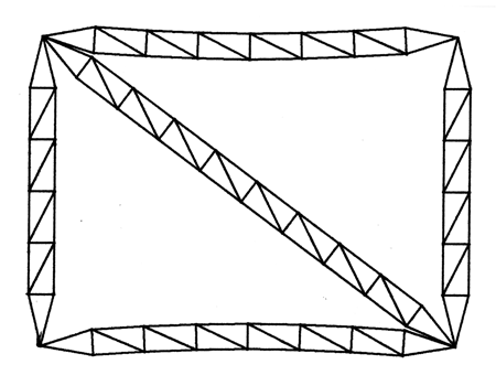
 w2 = 1.132 x 10⁻²
s-2
FIGURE 6.6 THE 'NEWBAR10' OBJECT
SECOND NONZERO MODE
w2 = 1.132 x 10⁻²
s-2
FIGURE 6.6 THE 'NEWBAR10' OBJECT
SECOND NONZERO MODE
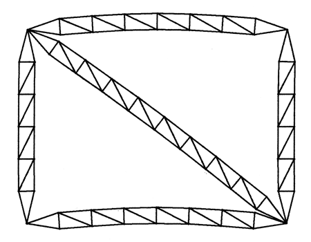
 w2 = 3.312 x 10⁻²
s-2
FIGURE 6.7 THE 'NEWBAR10' OBJECT
THIRD NONZERO MODE
w2 = 3.312 x 10⁻²
s-2
FIGURE 6.7 THE 'NEWBAR10' OBJECT
THIRD NONZERO MODE
Having obtained some results for this object, we can now use
it to build something new, say for instance a square frame. The objects 'newbar6'
and 'newbar8' are similar to 'newbar10' but shorter in length. Their object
descriptions are omitted for brevity.
( PROBLEM
( OBJECT bigsquare
( TOPOLOGY
( SUBOBJECTS 5
( subobj name)
(
( 0 newbar6 )
( 1 newbar8 )
( 2 newbar10 )
( 3 newbar8 )
( 4 newbar6 )
)
)
( NODES 4
(
(0 0.00 0.00 0.00)
(1 0.00 6.00 0.00)
(2 8.00 0.00 0.00)
(3 8.00 6.00 0.00)
)
)
( INCIDENCES 5
( subobj incidences)
(
(0 0 1)
(1 0 2)
(2 1 2)
(3 1 3)
(4 2 3)
)
)
)
)
)
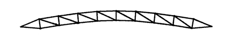
 6 levels of recursion
FIGURE 6.8 THE 'BIGSQUARE'
OBJECT
6 levels of recursion
FIGURE 6.8 THE 'BIGSQUARE'
OBJECT
 w2 = 3.841 x 10⁻⁴s-2
FIGURE 6.9 THE 'BIGSQUARE'
OBJECT FIRST NONZERO MODE
w2 = 3.841 x 10⁻⁴s-2
FIGURE 6.9 THE 'BIGSQUARE'
OBJECT FIRST NONZERO MODE
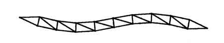
 w2 = 7.354 x 10⁻⁴s-2
FIGURE 6.10 THE 'BIGSQUARE'
OBJECT SECOND NONZERO MODE
w2 = 7.354 x 10⁻⁴s-2
FIGURE 6.10 THE 'BIGSQUARE'
OBJECT SECOND NONZERO MODE
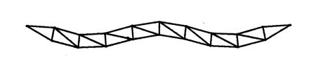
 w2 = 1.135 x 10⁻³s-2
FIGURE 6.11 THE 'BIGSQUARE'
OBJECT THIRD NONZERO MODE
w2 = 1.135 x 10⁻³s-2
FIGURE 6.11 THE 'BIGSQUARE'
OBJECT THIRD NONZERO MODE
CHAPTER 7
CONCLUSIONS
Up to now, many computer graphicists have focused on
providing realistic looking images as opposed to finite element workers
who have focused on generating realistic responding structural system
results. The time has come to unify these diciplines so that objects in simulations
look and respond realistically. The test-bed development was initiated
with these ideas in mind.
The techniques used to develop the test-bed represent a top-down,
structured programming approach to
the problem of providing an environment in which new algorithms
may be tested. The codes that comprise the test-bed represent a versatile
research tool for the evaluation of substructuring and other finite element
algorithms as well as the generation of useful data for engineering simulations.
BIBLIOGRAPHY
[BATH82] Bathe, K. J., Finite Element Procedures in Engineering
Analysis, Prentice-Hall, Englewood Cliffs, N.J., 1982.
[BENF71] Benfield, W.A. and Hruda, R.F., "Vibration Analysis
of Structures by Component Mode Substitution", AIAA Journal, Vol. 9,
No. 7, 1971, pp. 1255-1261.
[BERM73] Berman, A., "Vibration Analysis of Structural Systems
Using Virtual Substructures", Shock and Vibration Bulletin, Proc. 43,
No. 2, 1973, pp. 13-22.
[CHUR41] Church, A. "The Calculi of Lambda Conversion", Annals
of Mathematical Studies 6, Princeton University Press 1941, Reprinted
by Klaus Reprint Co., 1965
[COHE82] Cohen E., "Subdivision Methods for Curves and Surfaces",
Tutorial Notes: Freeform Surfaces, 1982 ACM SIGGRAPH
[COOK81] Cook R.D., Concepts and Applications of Finite
Element Analysis, John Wiley & Sons, New York, 1981.
[CRAI77] Craig, R.R. Jr. and Chung, C.J., "Substructure Coupling
for Dynamic Analysis and Testing", NASA CR-2781, February 1977.
[DATE76] Date, C. J. Introduction to Database Management
Systems, Third Edition Addison-Wesley, 1981, Reading, Mass.
[DODD80] Dodds, R.H. Jr. and Lopez, L.A., "A Generalized Software
System for Non-linear Analysis", Advanced Engineering Software, Vol.
2, No. 4, 1980, pp. 161-168.
[DODD82] Dodds, R.H. Jr., Rehak, D.R. and Lopez, L.A., "Development
Methodologies for Computationally Oriented Scientific Software", Unpublished
Report, 1982.
[DOWE72] Dowell, E.H., "Free Vibration of an Arbitrary Structure
in Terms of Component Modes", Journal of Applied Mechanics, Vol. 39,
1972, pp. 727-732.
[FELI81] Felippa, C. A. Architecture of a Distributed Analysis
Network for Computational Mechanics Computers & Structures, 1981,
Vol. 13, pp. 405-413.
[HALE80] Hale, A.L. and Meirovitch, L., "A General Substructure
Synthesis Method for the Dynamic Simulation of Complex Structures", Journal
of Sound and Vibration, Vol. 69, No. 2, 1980, pp. 309-326.
[HALE82a] Hale, A.L. and Meirovitch, L., "A Procedure for Improving
Discrete Substructure Representation in Dynamic Synthesis", AIAA Journal,
Vol. 20, No. 8, 1982, pp. 1128-1136.
[HALE82b] Hale, A.L., "A Family of Subspace Iteration Algorithms
for the Eigensolution of Large Structural Systems Composed of Substructures",
Proceedings of the First International Modal Analysis Conference, Orlando,
Florida, November 8-10, 1982, pp. 500-507.
[HINT75] Hintz, R.M., "Analytical Methods in Component Mode
Synthesis", AIAA Journal, Vol. 13, 1975, pp. 1007-1016.
[HURT65] Hurty, W.C., "Dynamic Analysis of Structural Systems
Using Component Modes", AIAA Journal, Vol. 3, No. 4, 1965, pp. 678-685.
[JENN77] Jennings, A., Matrix Computation for Engineers
and Scientists, John Wiley & Sons, New York, 1977.
[JOHN78] Johnson, S.C., "Yacc: Yet Another Compiler-Compiler",
Internal Document, Bell Laboratories, Murray Hill, N.J., 1978.
[LESK75] Lesk, M.E. and Schmidt E., "Lex - A Lexical Analyzer
Generator", Internal Document, Bell Laboratories, Murray Hill, N.J., 1975.
[LOPE82] Lopez, L.A., Dodds, R.H. Jr. and Rehak, D.R., "FINITE-Design
Concepts, Features and Capability", Unpublished Report, February, 1982.
[MACN71] MacNeal, R.H., "A Hybrid Method of Component Mode
Synthesis", Computers and Structures, Vol. 1, 1971, pp. 581-601.
[MEIR80] Meirovitch, L., Computational Methods in Structural
Dynamics, Sijthoff-Noordhoff International Publishers, Alphen ann den
Rijn, The Netherlands, 1980.
[MEIR81] Meirovitch, L. and Hale, A.L., "On the Substructure
Synthesis Method", AIAA Journal, Vol. 19, No. 7, 1981, pp. 940-947.
[NOOR78] Noor, A.K., Kamel, H.A. and Fulton, R.E., "Substructuring
Techniques, Status and Projections", Computers and Structures, Vol.
8, 1978, pp. 621-632.
[PARL80] Parlett, B. N., The Symmetric Eigenvalue Problem,
Prentice-Hall, Englewood Cliffs, N.J., 1980.
[PETE77] Petersson, H. and Popov, E.P., "Substructuring and
Equation System Solutions in Finite Element Analysis", Computers and Structures,
Vol. 7, 1977, pp. 197-206.
[PRZE63] Przemieniecki, J.S., "Matrix Structural Analysis of
Substructures", AIAA Journal, Vol. 1, 1963, pp. 138-147.
[REYN78] Reynolds, C. "Computer Animation in the World of Actors
and Scripts", SM thesis, MIT (Architecture Machine Group), May 1978
[REYN82] Reynolds, C. "Computer Animation with Scripts and
Actors", Computer Graphics 1982, Vol. 16, No. 3, pp. 289-296
[SCHR79] Schrem, E., "Trends and Aspects of the Development
of Large Finite Element Software Systems", Computers and Structures,
Vol. 10, 1979, pp. 419-425.
[WINO74] Winograd, T., Understanding Natural Language,
Academic Press, 1974.
[WINS81] Winston, P. and Horn, B., Lisp, Addison-Wesley,
1981.
[WHIT81] Whitted, T. and Weimer, D. M., "A Software Test-Bed
for the Devlopment of 3-d Raster Graphics Systems", Computer Graphics
Vol. 15, No. 3, 1981, pp. 271-277.
[ZIEN77] Zienkiewicz, O. C., under The Finite Element Method,
McGraw-Hill Book Company, United Kingdom, Ltd., 1977.