Abstract
The Designer's Desktop combines two of the engineer's most valuable tools: the engineer's handbook and the preprogrammed calculator. Merging these tools automates routine engineering tasks that would normally be tedious and time consuming. Section I of the Designer's Desktop contains BeamCALCulators for finding the shear, bending, deflections, shape, and stress. These quantities may be discovered rapidly for hollow and solid beams of rectangular, circular and I-beam cross sections. BeamCALCulators solve concentrated and distributed load problems for simply-supported and cantilevered beams.

Introduction and Overview
Engineers, scientists, and students have relied on bound paper handbooks for many years as quick references for frequently performed calculations, formulae, and engineering data. Easy to use computational equivalents of these handbooks have been hard to find. With problem solution techniques abounding, it is no longer so much an issue of whether a particular problem can be solved. The current issue is now the speed with which problems can be solved, not just by machine, but in toto. In a traditional setting, one is sidetracked by executing the following:

1) stop what one is doing,
2) find the relevant handbook,
3) read & understand the topic of interest..
4) transfer problem to computer.
5) pose the problem
6) solve the problem
7) vary the parameters
8) go to 6 until satisfied
9) return from sidetrack

This process can take days, weeks or months. The goal of this work is to shorten this problem-solving cycle to the minimum possible time, and while allowing for a high degree of quality control and accuracy.

A Traditional Example
As an example consider the frequent but mundane problem of a simply supported beam subjected to a distributed load:

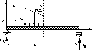
Definitions

L = beam length
a = x coordinate of load start
b = x coordinate of load end (0 < a < b < L)
Ra = the reaction at support A
Rb = the reaction at support B
wm = slope of spanwise load function
wb = intercept of spanwise load function
y(x) = deflection as a function of x
V(x) = shear as a function of x
M(x) = bending moment as a function of x

The subscripts of '1', '2' and '3' refer to the intervals 0 < x < a, a < x < b, and b < x < L respectively.

Summing Forces
Forces and moments are summed to deduce the values of the reactions at supports A and B:

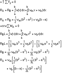
To perform the same derivation automatically we would say:

forcesEqn =
RA + RB - Integrate[wm x + wb , {x, a, b}] == 0;

momentEqn =
RB L - Integrate[wm x^2 + wb x, {x, a, b}] == 0;

reactions =
Solve[{forcesEqn, momentEqn},{ RA, RB }] ];

which yields:

RA =
(-a + b + (a^2 - b^2)/(2*L))*wb +
(-(a^2)/2 + b^2/2 + (a^3 - b^3)/(3*L))*wm

RB =
((-(a^2) + b^2)*wb)/(2*L) + ((-a^3 + b^3)*wm)/(3*L)

In the BeamCALCulators these expressions are incorporated into a pleasant interface for instant evaluation under varying conditions. This will be seen below.

Shear and Bending
We have the reactions in terms of the load distribution and beam length. We also seek shear, bending, deflection and end slopes.

For shear we have:

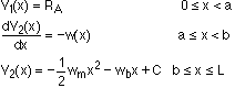
To find the value of C above, we must study the behavior of the shear as we cross the boundary of x = a. We know that for x < a the free body diagram yields the result that V1(x) = RA. After more algebra and taking limits:

Integrating onwards for bending the polynomials become more complex. At this stage, it is worth noting that small increases in expression complexity can cause symbolic manipulation programs to slow down dramatically. The phenomenon is due to a phenomenon called, "intermediate expression swell". It could just as well be termed, " stomach shrinkage" in the real one. The simplified symbolic manipulation versions of the shear and bending equations are:

shear1 = V1[x] -> Ra;

bending1 = {M1'[x] == V1[x] /. shear1};

bending1 = DSolve[bending1, M1[x], x];

Slope and Displacement
To compute spanwise deflection and slope, we refer to linear bending theory which states:

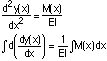
This is assuming constant stiffness along the length of the beam.
Utilizing this relation produces three slope expressions, one for each interval, which can be evaluated at the endpoints x =0 and x=L to provide the end slopes. These three slope expressions can be further integrated to give the displacement functions that describe the shape of the beam.

If we were smart, we would go to lunch. Not because these expressions are complex, no, rather because they are linked by six constants of integration, that are difficult to solve for by hand. We forge on. The cafeteria doesn't close till 1:30.

For the second interval a<x<b we have:

dy2dx'[x] == M2[x]/(EI) /. bending2;

slope2 =
DSolve[%, dy2dx[x], x] /. C[1] -> C1p;

y2'[x] == Last[slope2];

displacement2 =
DSolve[%, y2[x], x] /. C[1] -> C2p;

The result of which is:

dy2dx[x]=
C1p + (x*(-12*a^2*wb - 8*a^3*wm + 12*Ra*x + 12*a*wb*x + 6*a^2*wm*x - 4*wb*x^2 - wm*x^3))/(24*(E*I))

y2[x]=
C2p + C1p*x + (x^2*(-30*a^2*wb - 20*a^3*wm + 20*Ra*x + 20*a*wb*x + 10*a^2*wm*x - 5*wb*x^2 - wm*x^3))/(120*(E*I))

Simultaneous Solution
Having completed our slope and displacement integration we still have to solve for the constants. This turns out to be quite a bit of work if done by hand. The equations are:

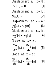
These equations look innocent until one tries to solve them. It even takes the computer awhile. In fact, it takes the computer the whole lunch hour! Now we can, should, and do, go to lunch. We leave the machine running the following math:

bc1 = displacement1 /. x->0 /. y1[0]->0 ;
bc2 = displacement3 /. x->L /. y3[L]->0 ;
bc3 = ( ( (displacement1 /. x-> a) -
displacement2 /. x-> a) ) == 0 ;
bc4 = ( ( ( slope1 /. x-> a) -
slope2 /. x-> a) ) == 0 ;
bc5 = ( ( (displacement2 /. x-> b) -
displacement3 /. x-> b) ) == 0 ;
bc6 = ( ( ( slope2 /. x-> b) -
slope3 /. x-> b) ) == 0 ;
constants =
Solve [ {bc1, bc2, bc3, bc4, bc5, bc6},
{C1, C2, C1p, C2p, C1pp, C2pp} ];

On returning from lunch, we find the problem still running. Just as we're about to cancel the job, out pop a page full of constants that solve the linked equations. These need to be transferred to a spreadsheet. We also need a user interface. With all these additions we miss lunch tomorrow too! Or, we could hope for a more complete version.
BeamCALCulator Examples
The problem whose solution we just derived can be solved in seconds with the BeamCALCulator. We start out by selecting the material from a table consisting of common metals, alloys, plastics. Custom materials can also be defined.

The material table contains the name, elastic, modulus, yield strength, specific weight and strength to weight ratio.

After a suitable material selection has been made, the cross section is specified as solid or hollow, square, elliptical or flanged. Exact dimensions are supplied and the section properties are computed.

Finally, the load is specified. This requires supplying the beam length, load beginning, load end, and load slope. At this point, a dynamic visual diagram is instantly updated.

Benefits
A benefit of casting common handbook problems into this format, is that designers, engineers and other interested parties can develop intuition with real structures in various loading conditions. This ability to instantly simulate the effect of different material, shape and load choices replaces thousands of possible physical experiments, enabling optimization of the structure and an accompanying reduction in cost and time.

Verification
BeamCALCulators are verified by comparison with different solution techniques and published example problems. An interesting outcome of the development of this software is that numerous errors have been uncovered in existing handbook formulae. Everyone is fallible, however, and it would be wise to assume that BeamCALCulators could contain errors. Because of human error, both in development, as well as in utilization, no warranty of fitness for any purpose is expressed or implied, and the user assumes all risk and responsibility arising from the use of the software.

Distribution
The BeamCALCulators, unlike their physical counterparts are software and therefore pure information. This enables electronic distribution through a variety of online network services including America Online and the internet. The software is also distributed in traditional disk formats.

Hardware/Software Platforms
BeamCALCulators run on top of Microsoft Excel. Any machine that runs Microsoft Excel or Office can host Designer's Desktop products.

Conclusions
Real world experiments are still necessary to characterize material properties, but are not necessary for every possible variation in problem parameters. This approach can be applied to a whole host of specific problems in various engineering areas. Section II of the Designer's Desktop performs conversion between various units and dimensions. Future sections will address additional engineering areas.

References
Wolfram, Stephen with Beck, George. Mathematica: the student book, Addison Wesley New York, NY, 1994

Microsoft Excel User's Guide Microsoft Corporation Redmond, WA 98052 1995

AIAA Aerospace Design Engineer Guide American Institute of Aeronautics and Astronautics, New York, NY 1987

Beer, Ferdinand P. and Johnston, E. Russell Jr. Vector Mechanics for Engineers Third Edition McGraw-Hill New York, NY 1977

Hibbeler, Russell C. Mechanics of Materials Second Edition Prentice-Hall Englewood Cliffs, NJ 1994

Tapley, Byron D. editor Eshbach's Handbook of Engineering Fundamentals Fourth Edition, John Wiley & Sons 1990