Determine the spanwise load constants in the distributed load equation:

in terms of the wing span, root chord, rip chord and applied load.

Solution:
Let:
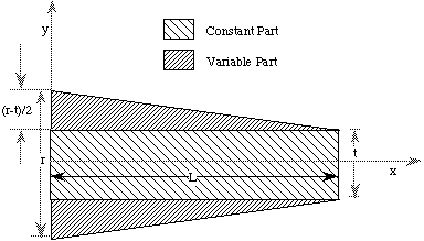
L = half span of wing from root to tip.
r = root chord
t = tip chord
Ac = region of constant load per unit length
Av = region of varying load per unit length
Aw = Ac + Av = total wing area
Wc = load in Ac
Wv = load in Av
W = total applied load
wc(x) = load as a function of x in constant region.
wv(x) = load as a function of x in varying region.
w(x) = wc(x) + wv(x) = total spanwise load
wm = slope of spanwise load function
wb = intercept of spanwise load function.

We will solve the problem in two parts. First we will find the portion of the load that does not vary with span, this will be called wc(x) where the subscript 'c' stands for constant. Then we will find the varying part of the load, called wv(x) where 'v' stands for variable. The following diagram will help us divide the problem into these two parts:

First :

Proof:

Next :

Proof:

Now we must formulate the load distribution in two parts, for the constant region and the varying region. We'll start with the constant case. We know that its graph looks like:

But all that we can establish from this is that:

However, we do know that this portion of the distributed load must sum to , which gives us a basis for finding the value of the unknown k:

Having solved the problem for the constant region we can now turn our attention to the varying one. We know that the linear taper in the wing gives rise to a linearly varying load whose graph is as follows:

The equation of this load function looks like this:

Again we are in the position of having to deduce the value of an unknown constant, in this case . To do this we again refer to the fact that the total area of the load curve must equal :

To solve the original problem, that is finding the slope and intercept of the combined load we add the two load distribution functions:

but we want to factor things like so:

where:

and:

which when boiled down and substituted gives:

which is fairly simple compared to the intermediate expression swell we suffered to get it.